thresholds <- seq(0.01, 0.30, by = 0.005)
n_test_obs <- nrow(test_data)
y_test <- test_data$readmitted
prev <- mean(y_test)
calc_nb <- function(probs, y, thresholds) {
n <- length(y)
vapply(thresholds, function(pt) {
pred_pos <- probs >= pt
tp <- sum(y == 1 & pred_pos)
fp <- sum(y == 0 & pred_pos)
(tp / n) - (fp / n) * (pt / (1 - pt))
}, numeric(1))
}
nb_all <- prev - (1 - prev) * (thresholds / (1 - thresholds))
dca_df <- bind_rows(
data.frame(
threshold = thresholds,
net_benefit = calc_nb(test_data$nb_pred, y_test, thresholds),
label = "NB Model"
),
data.frame(
threshold = thresholds,
net_benefit = calc_nb(test_data$adj_nb_pred, y_test, thresholds),
label = "Adjusted NB Model"
),
data.frame(
threshold = thresholds,
net_benefit = calc_nb(test_data$bw_pred, y_test, thresholds),
label = "Backward elimination"
),
data.frame(
threshold = thresholds,
net_benefit = calc_nb(test_data$lasso_pred, y_test, thresholds),
label = "LASSO"
),
data.frame(
threshold = thresholds,
net_benefit = nb_all,
label = "Treat all"
),
data.frame(
threshold = thresholds,
net_benefit = 0,
label = "Treat none"
)
)
# Compute costs per method
cost_nb <- NBvarsel:::calculate_model_cost(preds_best_nb, grouped_costs)
cost_adj <- NBvarsel:::calculate_model_cost(preds_best_adj, grouped_costs)
cost_bw <- NBvarsel:::calculate_model_cost(bw$names.kept, grouped_costs)
cost_lasso <- NBvarsel:::calculate_model_cost(lasso_kept, grouped_costs)
dca_df <- dca_df |>
mutate(
cost = case_when(
label == "NB Model" ~ cost_nb,
label == "Adjusted NB Model" ~ cost_adj,
label == "Backward elimination" ~ cost_bw,
label == "LASSO" ~ cost_lasso,
TRUE ~ 0
),
adj_net_benefit = net_benefit - cost
)
model_labels <- c(
"NB Model", "Adjusted NB Model", "Backward elimination",
"LASSO", "Treat all", "Treat none"
)
dca_df$label <- factor(dca_df$label, levels = model_labels)
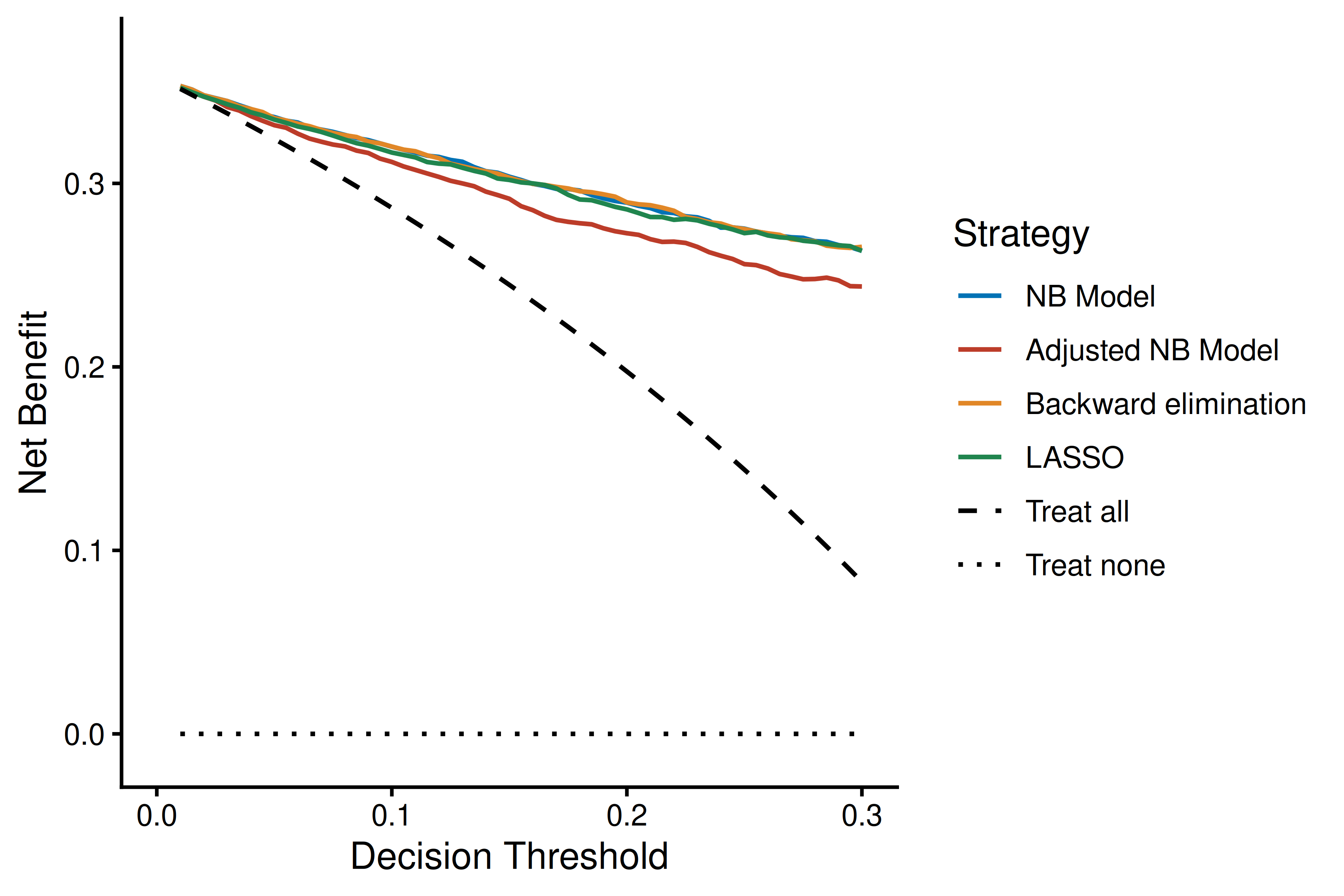
# Raw NB
ggplot(dca_df, aes(x = threshold, y = net_benefit, color = label, linetype = label)) +
geom_line(linewidth = 0.7) +
theme_classic(base_size = 12) +
labs(x = "Decision Threshold", y = "Net Benefit", color = "Strategy",
linetype = "Strategy") +
coord_cartesian(xlim = c(0, 0.30), ylim = c(-0.01, max(dca_df$net_benefit) * 1.05)) +
scale_color_manual(values = c(
"NB Model" = "#0072B5", "Adjusted NB Model" = "#BC3C29",
"Backward elimination" = "#E18727", "LASSO" = "#20854E",
"Treat all" = "black", "Treat none" = "black"
)) +
scale_linetype_manual(values = c(
"NB Model" = "solid", "Adjusted NB Model" = "solid",
"Backward elimination" = "solid", "LASSO" = "solid",
"Treat all" = "dashed", "Treat none" = "dotted"
))
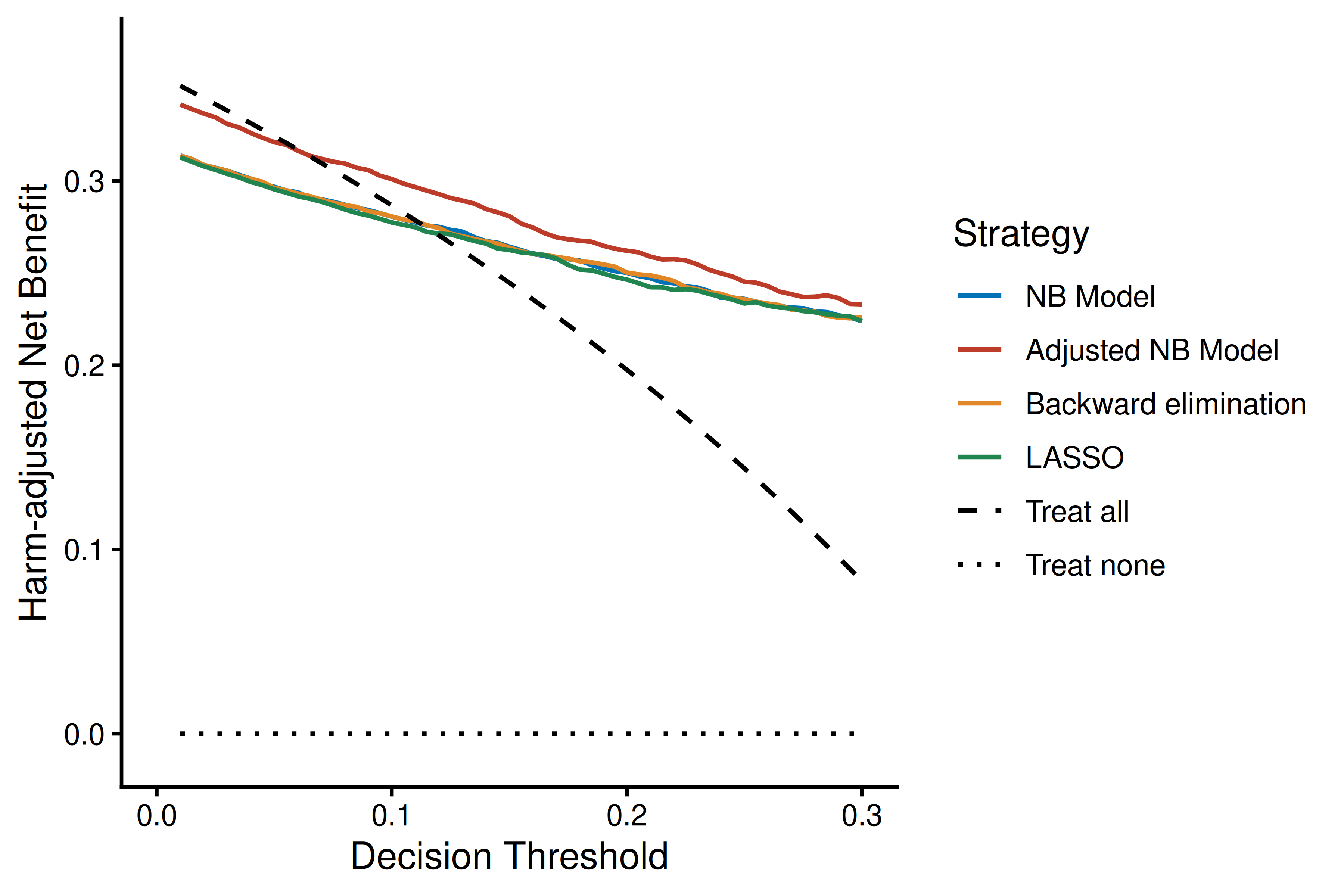
# Adjusted NB
ggplot(dca_df, aes(x = threshold, y = adj_net_benefit, color = label, linetype = label)) +
geom_line(linewidth = 0.7) +
theme_classic(base_size = 12) +
labs(
x = "Decision Threshold",
y = "Harm-adjusted Net Benefit",
color = "Strategy",
linetype = "Strategy"
) +
coord_cartesian(xlim = c(0, 0.30), ylim = c(-0.01, max(dca_df$adj_net_benefit) * 1.05)) +
scale_color_manual(values = c(
"NB Model" = "#0072B5", "Adjusted NB Model" = "#BC3C29",
"Backward elimination" = "#E18727", "LASSO" = "#20854E",
"Treat all" = "black", "Treat none" = "black"
)) +
scale_linetype_manual(values = c(
"NB Model" = "solid", "Adjusted NB Model" = "solid",
"Backward elimination" = "solid", "LASSO" = "solid",
"Treat all" = "dashed", "Treat none" = "dotted"
))